Create Calculated Field At PivotTable

Question:

How can I create a calculation from the total of a count of a field on a pivot table? Example: I need to calculate the number of employees for each process level times a specified amount - 89 x $4.59, 3 x $4.59.

Answer:
Select the table and click Insert, PivotTable. Drag the required field to relevant label (Refer the details of creating pivotTable at post Show Variance Between Year PivotTable). Create the pivotTable as Picture 1. To create a calculated field, click at the pivotTable and click Option, Formulas, Calculated Field.

Picture 1

A Insert calculated Field will show, type the name for the calculated field and type the formula, then click Add, click OK.

Picture 2

The calculated field will then created as following:

Show Variance Between Year PivotTable

Hi AJ,



Question:

I need to create a variance formula for the data selected in a pivot table.

My problem is that the data is coming in from one column and I don't know how

to distinquish the data by year in the formula. I have put a small selection

of my data below. I would like to show the variance between 2009 and 2010

for all months selected in the pivot table.
 
 
Answer:
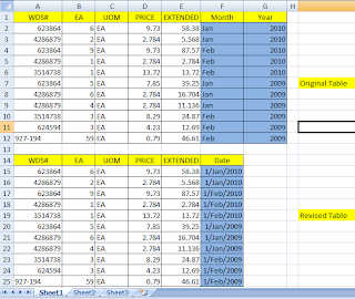
Base on the question and data, I summary it in the Original Table below (Picture 1). In order to show the variance between 2009 and 2010, I believe the better way is summary the Month and Year column into Date column as Revised Table below. With the Date column, you can manipulate the data into many way as you like as explanation below.
 

Picture 1

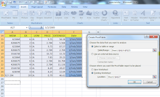
After you revised the table to Date column, you can select the table and click Insert, PivotTable. Select the appropriate option as Picture 2.

Picture 2



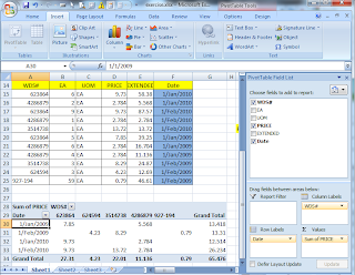
Simply drag the required fields to Columns Label, Row Labels, Values, or Report Filter at PivotTable Field list. The PivotTable will then created.

Picture 3

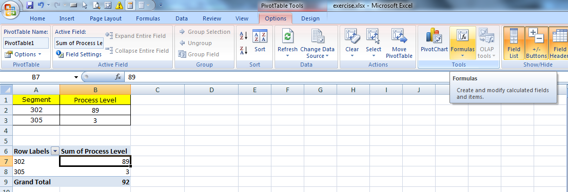
Now you can manipulate the PivotTable as you like. You can group the date by year. Click at the date field, right-click and select Group.

The Grouping message box will show. Make the selection. In this case, I want to group by Year, so select Years. Then click OK.



Now you can see the different of year 2009 and 2010. Hopefully it can solve your question. If not, do not hesitate to write your question at comment. Thank you.

Show Pie Chart By Month

You can show data into pie chart by month. By selecting a month, the pie chart will shown as picture below.

Instruction:

1) Data Validation is a good function to create a list of selection. You can use Data Validation to create a list of month as picture below.


2) Vlookup or Hlookup is a good function to obtain data from a table. After selecting a month, use Vlookup to obtain data from table below. Thats all. After select a month, the data from selected month will show at table above. Then, create pie chart using table above.

Compiling Data By Date

Some people maybe take time to combile all the data by date/week/month/year, actually PivotTable tool at Microsoft Excel is useful for combile the data in table by date/week/month/year and also plot in into chart.

Instruction:
1. Select the data, click Insert, PivotTable,select New Worksheet or Existing Worksheet,select location, OK.
2. The PivotTable Field List will then shown at the right, select the Date and Quantity field list, then the table will created.

Include a value from one cell within text of another cell.

Regarding the question when user enter data in cell B4, the cell B5 will show text such as " X is not a valid entry. Please enter the correct pair number." for entry of 25~150 (X is the enter number). You can use the formula below at cell B5:

You can also use Data Validation at Data, Data Validation by setting Setting below.

You can also set message box to display by setting Error Alert below.

When the number 25 to 150 is enter, a message box and text is displayed as below.

Conditional Formatting Date Range

Regarding the question how to use Conditional Formatting to look at the range of dates in
B3:B13 and highlight all the cells that contain a date in the mini calendar. You can use sumproduct formula in your conditional formatting. You can see the picture below, when you use sumproduct for cell Q7 compare with range B3:B13, it will equal to 1 because it is in the range.




Therefore, you can use the formula to conditional formatting's formula by setting it to red color if the formula more than o or equal 1.

Check box help in Word

Regarding the question of a faster way to do check/uncheck these boxes, I propose create a command button to perform you required action. To do this, you need to create a simple program to do this.

Follow the steps below:
1) Insert Checkbox (from Forms toolbar) and Commandbutton (from Control Toolbox). (For Word 2007, click Customize Quick Access Toolbar, More Command, Choose Command From: All Command, add Check box, Command button).
2) Select the Commandbutton and right-click to select View Code.

3) The Microsoft Visual Basic will open for you to write coding. Write this statement to enable the checkbox check after press command button.

ActiveDocument.FormFields("Check1").CheckBox.Value=True

4) Double-click the checkbox to ensure the check box name is tally.

5) Select the commandbutton and right-click to select CommandButton Object, Edit to change the commandbutton caption to "Check".

6) Click Exit Design Mode. Now you can click the "Check" button to check the checkbox. (For Word 2007, click Customize Quick Access Toolbar, More Command, Choose Command From: All Command, add Design Mode).

7) Now, when you click the button, the check box will check. You can also write other program to perform action required by you.